25. Cattle Cycles #

Contents

Cattle Cycles
- The Model
- Mapping into HS2013 Framework

This is another member of a suite of lectures that use the quantecon DLE class to instantiate models within the [Hansen and Sargent, 2013] class of models described in detail in Recursive Models of Dynamic Linear Economies.

In addition to what’s in Anaconda, this lecture uses the quantecon library.

!pip install --upgrade quantecon

Show code cell output Hide code cell output

Collecting quantecon

  Downloading quantecon-0.7.2-py3-none-any.whl.metadata (4.9 kB)

Requirement already satisfied: numba>=0.49.0 in /home/runner/miniconda3/envs/quantecon/lib/python3.11/site-packages (from quantecon) (0.59.0)
Requirement already satisfied: numpy>=1.17.0 in /home/runner/miniconda3/envs/quantecon/lib/python3.11/site-packages (from quantecon) (1.26.4)
Requirement already satisfied: requests in /home/runner/miniconda3/envs/quantecon/lib/python3.11/site-packages (from quantecon) (2.31.0)
Requirement already satisfied: scipy>=1.5.0 in /home/runner/miniconda3/envs/quantecon/lib/python3.11/site-packages (from quantecon) (1.11.4)
Requirement already satisfied: sympy in /home/runner/miniconda3/envs/quantecon/lib/python3.11/site-packages (from quantecon) (1.12)
Requirement already satisfied: llvmlite<0.43,>=0.42.0dev0 in /home/runner/miniconda3/envs/quantecon/lib/python3.11/site-packages (from numba>=0.49.0->quantecon) (0.42.0)
Requirement already satisfied: charset-normalizer<4,>=2 in /home/runner/miniconda3/envs/quantecon/lib/python3.11/site-packages (from requests->quantecon) (2.0.4)
Requirement already satisfied: idna<4,>=2.5 in /home/runner/miniconda3/envs/quantecon/lib/python3.11/site-packages (from requests->quantecon) (3.4)
Requirement already satisfied: urllib3<3,>=1.21.1 in /home/runner/miniconda3/envs/quantecon/lib/python3.11/site-packages (from requests->quantecon) (2.0.7)
Requirement already satisfied: certifi>=2017.4.17 in /home/runner/miniconda3/envs/quantecon/lib/python3.11/site-packages (from requests->quantecon) (2024.2.2)
Requirement already satisfied: mpmath>=0.19 in /home/runner/miniconda3/envs/quantecon/lib/python3.11/site-packages (from sympy->quantecon) (1.3.0)

Downloading quantecon-0.7.2-py3-none-any.whl (215 kB)
?25l   ━━━━━━━━━━━━━━━━━━━━━━━━━━━━━━━━━━━━━━━━ 0.0/215.4 kB ? eta -:--:--
   ━━━━━━━━━━━━━━━━━━━━━━━━━━━━━━━━━━━━━━━━ 215.4/215.4 kB 10.5 MB/s eta 0:00:00
?25h

Installing collected packages: quantecon

Successfully installed quantecon-0.7.2

This lecture uses the DLE class to construct instances of the “Cattle Cycles” model of Rosen, Murphy and Scheinkman (1994) [Rosen et al., 1994].

That paper constructs a rational expectations equilibrium model to understand sources of recurrent cycles in US cattle stocks and prices.

We make the following imports:

import numpy as np
import matplotlib.pyplot as plt
from collections import namedtuple
from quantecon import DLE
from math import sqrt

25.1. The Model #

The model features a static linear demand curve and a “time-to-grow” structure for cattle.

Let $p_{t}$ be the price of slaughtered beef, $m_{t}$ the cost of preparing an animal for slaughter, $h_{t}$ the holding cost for a mature animal, $γ_{1} h_{t}$ the holding cost for a yearling, and $γ_{0} h_{t}$ the holding cost for a calf.

The cost processes ${h_{t}, m_{t}}_{t = 0}^{\infty}$ are exogenous, while the price process ${p_{t}}_{t = 0}^{\infty}$ is determined within a rational expectations equilibrium.

Let $x_{t}$ be the breeding stock, and $y_{t}$ be the total stock of cattle.

The law of motion for the breeding stock is

x_{t} = (1 - δ) x_{t - 1} + g x_{t - 3} - c_{t}

where $g < 1$ is the number of calves that each member of the breeding stock has each year, and $c_{t}$ is the number of cattle slaughtered.

The total headcount of cattle is

y_{t} = x_{t} + g x_{t - 1} + g x_{t - 2}

This equation states that the total number of cattle equals the sum of adults, calves and yearlings, respectively.

A representative farmer chooses ${c_{t}, x_{t}}$ to maximize:

E_{0} \sum_{t = 0}^{\infty} β^{t} {p_{t} c_{t} - h_{t} x_{t} - γ_{0} h_{t} (g x_{t - 1}) - γ_{1} h_{t} (g x_{t - 2}) - m_{t} c_{t} - \frac{ψ_{1}}{2} x_{t}^{2} - \frac{ψ_{2}}{2} x_{t - 1}^{2} - \frac{ψ_{3}}{2} x_{t - 3}^{2} - \frac{ψ_{4}}{2} c_{t}^{2}}

subject to the law of motion for $x_{t}$ , taking as given the stochastic laws of motion for the exogenous processes, the equilibrium price process, and the initial state [ $x_{- 1}, x_{- 2}, x_{- 3}$ ].

Remark The $ψ_{j}$ parameters are very small quadratic costs that are included for technical reasons to make well posed and well behaved the linear quadratic dynamic programming problem solved by the fictitious planner who in effect chooses equilibrium quantities and shadow prices.

Demand for beef is government by $c_{t} = a_{0} - a_{1} p_{t} + {\tilde{d}}_{t}$ where ${\tilde{d}}_{t}$ is a stochastic process with mean zero, representing a demand shifter.

25.2. Mapping into HS2013 Framework #

25.2.1. Preferences#

We set $Λ = 0, Δ_{h} = 0, Θ_{h} = 0, Π = α_{1}^{- \frac{1}{2}}$ and $b_{t} = Π {\tilde{d}}_{t} + Π α_{0}$ .

With these settings, the FOC for the household’s problem becomes the demand curve of the “Cattle Cycles” model.

25.2.2. Technology#

To capture the law of motion for cattle, we set

\begin{array}{r} Δ_{k} = [\begin{array}{ccc} (1 - δ) & 0 & g \\ 1 & 0 & 0 \\ 0 & 1 & 0 \end{array}], Θ_{k} = [\begin{array}{c} 1 \\ 0 \\ 0 \end{array}] \end{array}

(where $i_{t} = - c_{t}$ ).

To capture the production of cattle, we set

\begin{array}{r} Φ_{c} = [\begin{array}{c} 1 \\ f_{1} \\ 0 \\ 0 \\ - f_{7} \end{array}], Φ_{g} = [\begin{array}{cccc} 0 & 0 & 0 & 0 \\ 1 & 0 & 0 & 0 \\ 0 & 1 & 0 & 0 \\ 0 & 0 & 1 & 0 \\ 0 & 0 & 0 & 1 \end{array}], Φ_{i} = [\begin{array}{c} 1 \\ 0 \\ 0 \\ 0 \\ 0 \end{array}], Γ = [\begin{array}{ccc} 0 & 0 & 0 \\ f_{1} (1 - δ) & 0 & g f_{1} \\ f_{3} & 0 & 0 \\ 0 & f_{5} & 0 \\ 0 & 0 & 0 \end{array}] \end{array}

25.2.3. Information#

We set

\begin{array}{r} A_{22} = [\begin{array}{cccc} 1 & 0 & 0 & 0 \\ 0 & ρ_{1} & 0 & 0 \\ 0 & 0 & ρ_{2} & 0 \\ 0 & 0 & 0 & ρ_{3} \end{array}], C_{2} = [\begin{array}{ccc} 0 & 0 & 0 \\ 1 & 0 & 0 \\ 0 & 1 & 0 \\ 0 & 0 & 15 \end{array}], U_{b} = [\begin{array}{cccc} Π α_{0} & 0 & 0 & Π \end{array}], U_{d} = [\begin{array}{c} 0 \\ f_{2} U_{h} \\ f_{4} U_{h} \\ f_{6} U_{h} \\ f_{8} U_{h} \end{array}] \end{array}

To map this into our class, we set $f_{1}^{2} = \frac{Ψ_{1}}{2}$ , $f_{2}^{2} = \frac{Ψ_{2}}{2}$ , $f_{3}^{2} = \frac{Ψ_{3}}{2}$ , $2 f_{1} f_{2} = 1$ , $2 f_{3} f_{4} = γ_{0} g$ , $2 f_{5} f_{6} = γ_{1} g$ .

# We define namedtuples in this way as it allows us to check, for example,
# what matrices are associated with a particular technology.

Information = namedtuple('Information', ['a22', 'c2', 'ub', 'ud'])
Technology = namedtuple('Technology', ['ϕ_c', 'ϕ_g', 'ϕ_i', 'γ', 'δ_k', 'θ_k'])
Preferences = namedtuple('Preferences', ['β', 'l_λ', 'π_h', 'δ_h', 'θ_h'])

We set parameters to those used by [Rosen et al., 1994]

β = np.array([[0.909]])
lλ = np.array([[0]])

a1 = 0.5
πh = np.array([[1 / (sqrt(a1))]])
δh = np.array([[0]])
θh = np.array([[0]])

δ = 0.1
g = 0.85
f1 = 0.001
f3 = 0.001
f5 = 0.001
f7 = 0.001

ϕc = np.array([[1], [f1], [0], [0], [-f7]])

ϕg = np.array([[0, 0, 0, 0],
               [1, 0, 0, 0],
               [0, 1, 0, 0],
               [0, 0, 1,0],
               [0, 0, 0, 1]])

ϕi = np.array([[1], [0], [0], [0], [0]])

γ = np.array([[           0,  0,      0],
              [f1 * (1 - δ),  0, g * f1],
              [          f3,  0,      0],
              [           0, f5,      0],
              [           0,  0,      0]])

δk = np.array([[1 - δ, 0, g],
               [    1, 0, 0],
               [    0, 1, 0]])

θk = np.array([[1], [0], [0]])

ρ1 = 0
ρ2 = 0
ρ3 = 0.6
a0 = 500
γ0 = 0.4
γ1 = 0.7
f2 = 1 / (2 * f1)
f4 = γ0 * g / (2 * f3)
f6 = γ1 * g / (2 * f5)
f8 = 1 / (2 * f7)

a22 = np.array([[1, 0, 0, 0],
                [0, ρ1, 0, 0],
                [0, 0, ρ2, 0],
                [0, 0, 0, ρ3]])

c2 = np.array([[0, 0,  0],
               [1, 0,  0],
               [0, 1,  0],
               [0, 0, 15]])

πh_scalar = πh.item()
ub = np.array([[πh_scalar * a0, 0, 0, πh_scalar]])
uh = np.array([[50, 1, 0, 0]])
um = np.array([[100, 0, 1, 0]])
ud = np.vstack(([0, 0, 0, 0],
                f2 * uh, f4 * uh, f6 * uh, f8 * um))

Notice that we have set $ρ_{1} = ρ_{2} = 0$ , so $h_{t}$ and $m_{t}$ consist of a constant and a white noise component.

We set up the economy using tuples for information, technology and preference matrices below.

We also construct two extra information matrices, corresponding to cases when $ρ_{3} = 1$ and $ρ_{3} = 0$ (as opposed to the baseline case of $ρ_{3} = 0.6$ ).

info1 = Information(a22, c2, ub, ud)
tech1 = Technology(ϕc, ϕg, ϕi, γ, δk, θk)
pref1 = Preferences(β, lλ, πh, δh, θh)

ρ3_2 = 1
a22_2 = np.array([[1,  0,  0,    0],
                  [0, ρ1,  0,    0],
                  [0,  0, ρ2,    0],
                  [0,  0,  0, ρ3_2]])

info2 = Information(a22_2, c2, ub, ud)

ρ3_3 = 0
a22_3 = np.array([[1,  0,  0,    0],
                  [0, ρ1,  0,    0],
                  [0,  0, ρ2,    0],
                  [0,  0,  0, ρ3_3]])

info3 = Information(a22_3, c2, ub, ud)

# Example of how we can look at the matrices associated with a given namedtuple
info1.a22

array([[1. , 0. , 0. , 0. ],
       [0. , 0. , 0. , 0. ],
       [0. , 0. , 0. , 0. ],
       [0. , 0. , 0. , 0.6]])

# Use tuples to define DLE class
econ1 = DLE(info1, tech1, pref1)
econ2 = DLE(info2, tech1, pref1)
econ3 = DLE(info3, tech1, pref1)

# Calculate steady-state in baseline case and use to set the initial condition
econ1.compute_steadystate(nnc=4)
x0 = econ1.zz

econ1.compute_sequence(x0, ts_length=100)

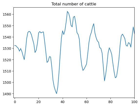
[Rosen et al., 1994] use the model to understand the sources of recurrent cycles in total cattle stocks.

Plotting $y_{t}$ for a simulation of their model shows its ability to generate cycles in quantities

# Calculation of y_t
totalstock = econ1.k[0] + g * econ1.k[1] + g * econ1.k[2]
fig, ax = plt.subplots()
ax.plot(totalstock)
ax.set_xlim((-1, 100))
ax.set_title('Total number of cattle')
plt.show()

_images/4aad3c16058c66dc03c10c85f7a2335d6a6000363e8ac40eb31da646f90858a2.png

In their Figure 3, [Rosen et al., 1994] plot the impulse response functions of consumption and the breeding stock of cattle to the demand shock, ${\tilde{d}}_{t}$ , under the three different values of $ρ_{3}$ .

We replicate their Figure 3 below

shock_demand = np.array([[0], [0], [1]])

econ1.irf(ts_length=25, shock=shock_demand)
econ2.irf(ts_length=25, shock=shock_demand)
econ3.irf(ts_length=25, shock=shock_demand)

fig, (ax1, ax2) = plt.subplots(1, 2, figsize=(12, 4))
ax1.plot(econ1.c_irf, label=r'$\rho=0.6$')
ax1.plot(econ2.c_irf, label=r'$\rho=1$')
ax1.plot(econ3.c_irf, label=r'$\rho=0$')
ax1.set_title('Consumption response to demand shock')
ax1.legend()

ax2.plot(econ1.k_irf[:, 0], label=r'$\rho=0.6$')
ax2.plot(econ2.k_irf[:, 0], label=r'$\rho=1$')
ax2.plot(econ3.k_irf[:, 0], label=r'$\rho=0$')
ax2.set_title('Breeding stock response to demand shock')
ax2.legend()
plt.show()

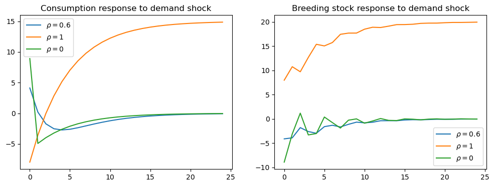
_images/acad5774b798f3feb756f82549bc87f8b900dd58b455f8377c5c7458dd977c46.png

The above figures show how consumption patterns differ markedly, depending on the persistence of the demand shock:

If it is purely transitory ( $ρ_{3} = 0$ ) then consumption rises immediately but is later reduced to build stocks up again.
If it is permanent ( $ρ_{3} = 1$ ), then consumption falls immediately, in order to build up stocks to satisfy the permanent rise in future demand.

In Figure 4 of their paper, [Rosen et al., 1994] plot the response to a demand shock of the breeding stock and the total stock, for $ρ_{3} = 0$ and $ρ_{3} = 0.6$ .

We replicate their Figure 4 below

total1_irf = econ1.k_irf[:, 0] + g * econ1.k_irf[:, 1] + g * econ1.k_irf[:, 2]
total3_irf = econ3.k_irf[:, 0] + g * econ3.k_irf[:, 1] + g * econ3.k_irf[:, 2]

fig, (ax1, ax2) = plt.subplots(1, 2, figsize=(12, 4))
ax1.plot(econ1.k_irf[:, 0], label='Breeding Stock')
ax1.plot(total1_irf, label='Total Stock')
ax1.set_title(r'$\rho=0.6$')

ax2.plot(econ3.k_irf[:, 0], label='Breeding Stock')
ax2.plot(total3_irf, label='Total Stock')
ax2.set_title(r'$\rho=0$')
plt.show()

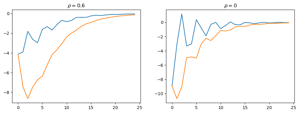
_images/f215d416e897904a4462af1ca1ecd441e654b96dfdad722100b2ed91444af8e1.png

The fact that $y_{t}$ is a weighted moving average of $x_{t}$ creates a humped shape response of the total stock in response to demand shocks, contributing to the cyclicality seen in the first graph of this lecture.

25. Cattle Cycles#

25.1. The Model#

25.2. Mapping into HS2013 Framework#